How Transportation Engineers Achieved 6.6cm Underwater Mapping Accuracy With Drones Powered by SPH Engineering Kit

The Challenge

North Carolina Department of Transportation needed to validate whether drone-mounted sonar could deliver the accuracy required for infrastructure planning. Traditional survey methods face limitations: boat-based multibeam sonar requires trained hydrographic surveyors and struggles in shallow or debris-filled water, while topographic LiDAR cannot penetrate water surfaces.

The research question: Can a drone-mounted single-beam sonar system achieve centimeter-level accuracy for transportation infrastructure assessment?\

The Research Project

Lead Organizations:

• Mississippi State University (primary research)
• Appalachian State University (supplementary North Carolina sites)

Project Scope: NCDOT Research Project 2024-32, January 2024 - March 2025

Sites Surveyed:

• Mississippi State: 7 locations across Mississippi (catfish ponds, lakes, rivers, coastal bays, irrigation reservoirs)
• Appalachian State: 4 North Carolina sites (Price Lake, Rhodhiss Lake, Huffman Bridge, Watauga River)

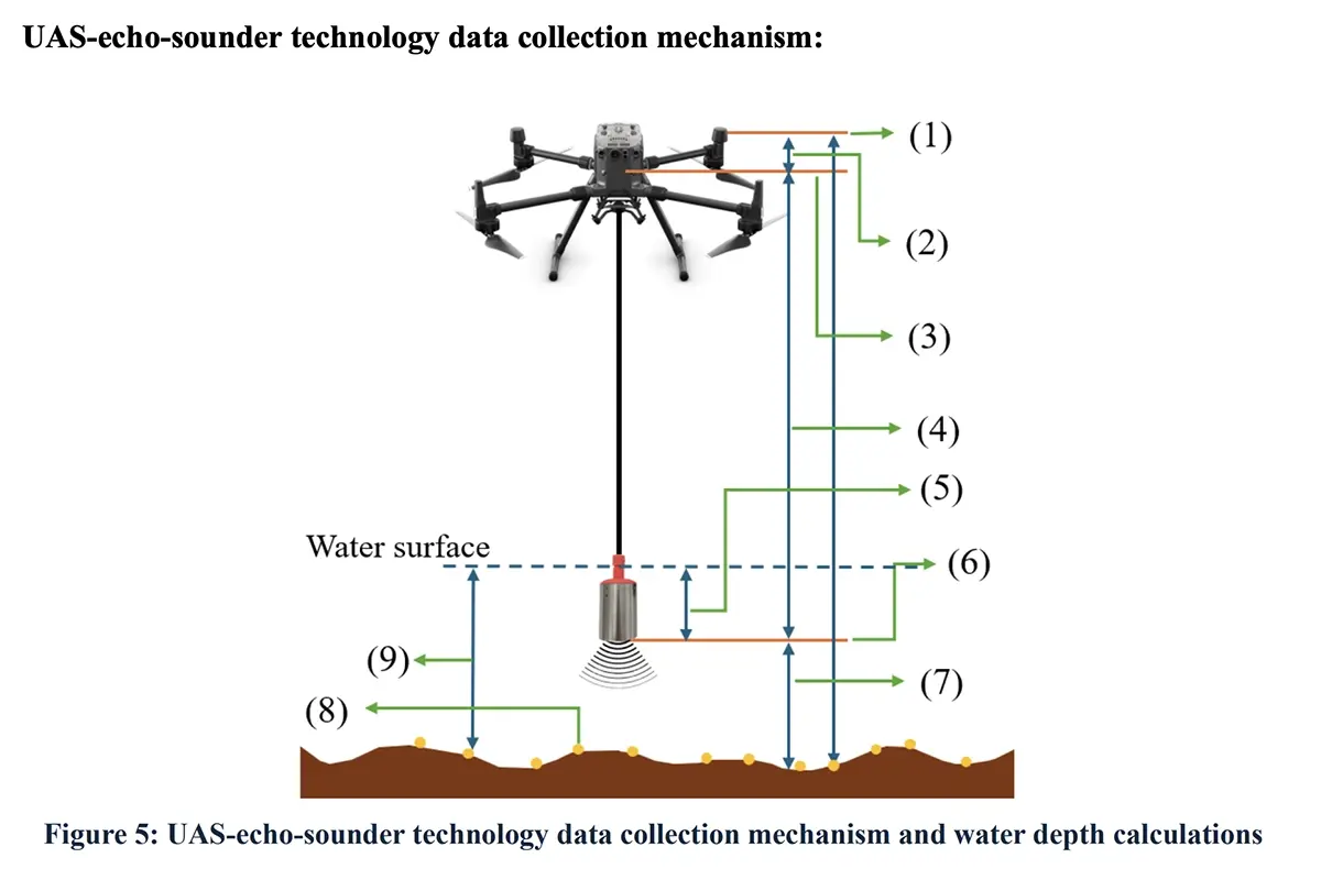
The Technical Problem: Eliminating Barometric Altimeter Drift

Single-beam sonar mounted on a drone measures the distance from the sensor to the underwater bottom. To calculate accurate bottom elevations, you need two precise measurements:

1. Drone altitude above the water surface
2. Sonar depth reading

The math: Bottom Elevation = Water Surface Elevation - Sonar Depth + Drone Altitude

Standard DJI drones use barometric altimeters that drift several meters during flight. That altitude error propagates directly into depth calculations, making the data unusable for engineering decisions.

The Solution: Precision Altitude Control with SPH Engineering SkyHub

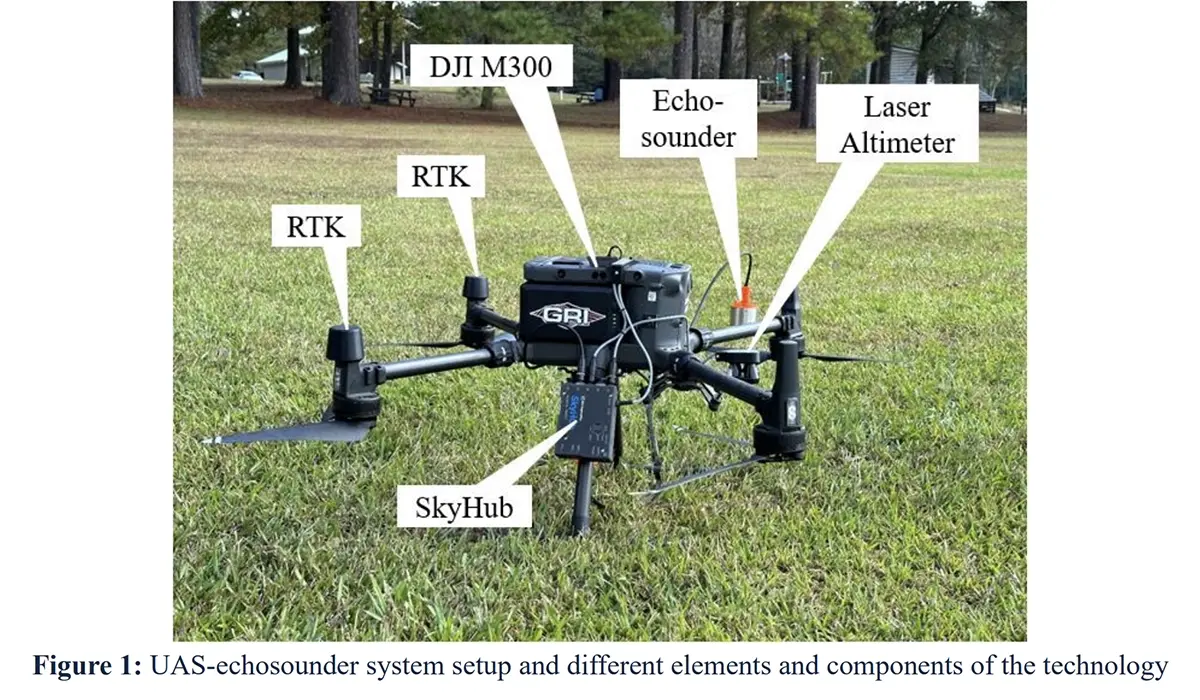
Hardware Integration

Drones Used:

• Mississippi State: DJI M300 RTK
• Appalachian State: DJI M600 Pro
• System also supports: DJI M210, Pixhawk-based drones

Echo Sounders:

• Mississippi State: ECT D052S dual-frequency (0.5m to 200m range, 0.2% depth accuracy)
• Appalachian State: ECT 400S single-frequency

Required Components:

• Stainless steel protection housing for sensor
• Cable set
• Hook and carabiner to attach sensor
• Radar or laser altimeter with drone mountings
• UgCS SkyHub onboard computer

Altitude Control: For this project, teams used a laser altimeter with a terrain/surface tracking algorithm. SPH Engineering SkyHub supports both radar and laser altimeters. The research report notes that radar altimeter configuration achieves "altitude stability with a drift of only about 5 cm" compared to several meters with standard barometric systems.

How UgCS SkyHub Works

Function 1: Precision Altitude Control

UgCS SkyHub maintains constant drone height above the water surface by reading data from the altimeter (radar or laser). The laser altimeter with surface tracking algorithm used in this project maintained consistent altitude throughout flights.

The report states: "Unlike standard DJI drones, which rely on less precise barometric altimeters and can experience altitude drifts of several meters during a single flight, the radar altimeter ensures altitude stability with a drift of only about 5 cm."

This altitude precision is what enables accurate depth calculations.

Function 2: Geotagged Data Logging

SkyHub uses the drone's GPS receiver (or RTK/PPK if equipped) to geotag every sonar ping with centimeter-level positioning. The system stores data in three formats:

• CSV: Coordinates, depth, metadata (works with Surfer, Oasis Montaj, Excel)
• NMEA 0183: Standard format for HydroMagic and Reefmaster hydrographic software‍
• SEG-Y: Full echo sounder waveform data for advanced analysis

Data logging starts automatically when the sonar detects water. No manual triggering required.

Function 3: Real-Time Monitoring

The ground control station displays live depth readings during flight. Operators can spot data quality issues immediately and adjust flight parameters if needed.

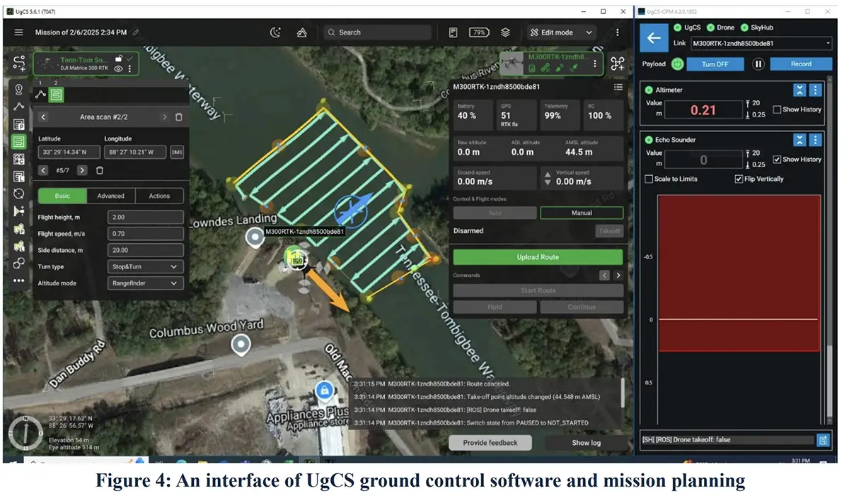
Mission Planning in UgCS

The Appalachian State team documented their workflow:

Planning Process

1. Import the survey area boundary KML into the UgCS desktop software
2. Plan the flight using the UgCS Area Scan algorithm (teams tested 5m, 10m, 20m, 30m line spacing)
3. Select operational mode (Continuous, Waypoint "grasshopper", or Manual)
4. Set flight speed and altitude
5. Configure Custom Payload Manager (CPM) for sonar ping rate and data storage

Flight Modes Available

UgCS offers three operational modes for bathymetric surveys:

• Continuous mode: Smooth parallel lines covering the survey area with the sensor submerged all the time
• Waypoint "grasshopper" mode: Point-by-point measurement approach involving submerging echosounder for each measurement point 
• Manual mode: Pilot-controlled flight with SkyHub data logging
• This research primarily used continuous parallel line mode for systematic coverage.

Speed Guidance

The research report recommends 0.5-0.7 m/s flight speed for stable sonar positioning in continuous mode. Appalachian State University flew at 0.8 m/s (noted as "recommended by SPH") and maintained good data quality with stable sensor tilt angles.

Results: Validating 6.6cm Vertical Accuracy (RMSE)

Mississippi State established a validation site at a catfish pond with known depth measurements from LiDAR and GNSS ground truth surveys.

Raw Performance (46,832 data points)

• Root Mean Square Error: 10.20 cm
• R² correlation: 72.8%

Filtered Performance (95.45% of data retained after 2 standard deviation filter)

• Root Mean Square Error: 6.59 cm
• R² correlation: 86.6%

This represents centimeter-level accuracy validated against LiDAR and GNSS reference datasets.

Error Patterns

The research team observed: "Most of the locations are shallower areas...where the error values are high, alternatively in deeper regions where there is more depth there are fewer outliers."

Sonar performs better in deeper water. Shallow areas under 0.5m showed higher error rates due to surface reflections and sensor range limitations.

Field Operations Across Different Water Types

Mississippi State Survey Sites

Bay Springs Lake (7.04 acres, freshwater lake)

• Flight time: 60 minutes
• Flight line spacing: 20m
• Batteries: 3 flight sessions
• Conditions: Calm water, optimal
• Result: Clean, consistent data

The team notes: "We faced a configuration issue on our first flight and lost our first set of battery power" - documenting real operational challenges.

Tombigbee River (8.11 acres, flowing water)

• Flight time: 70 minutes
• Flight line spacing: 20m
• Batteries: 3.5 flight sessions
• Conditions: Moving water, variable turbidity
• Result: More noise than still water but usable data

Grand Bay + Middle Bay (15.42 acres, coastal saltwater)

• Flight time: 120 minutes across 2 days
• Flight line spacing: 10m
• Batteries: 6 flight sessions
• Conditions: Saline water, tidal influence, wave action
• Access: Required boat transport to survey area

The team explains: "we initially had only four battery sets, [but] the two-day timeframe allowed us to recharge the additional two sets for use on the second day."

White's Creek Lake (5.04 acres, reservoir)

• Flight time: 40 minutes
• Flight line spacing: 10m
• Batteries: 2 flight sessions
• Conditions: Agricultural runoff, potential sedimentation
• Result: Successful mapping in shallow reservoir

Appalachian State Survey Sites (North Carolina)

Price Lake

During data collection: "watching the live sonar feed in UGCS we witnessed a large amounts of spikes and erroneous readings" - the real-time monitoring capability allowed operators to identify data quality issues during flight and understand why some areas showed sparse point coverage.

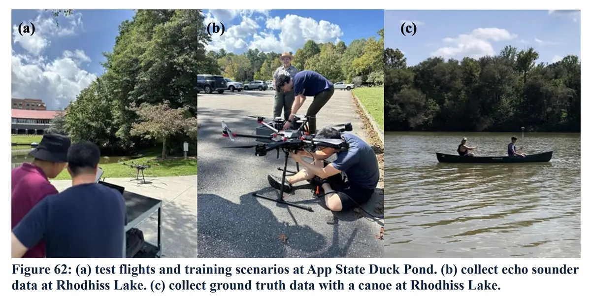
Rhodhiss Lake (Post-Hurricane Assessment)

The team conducted before-and-after surveys around Hurricane Helene:

• Pre-storm survey: August 22, 2024
• Post-storm survey: November 1, 2024

The autonomous flight path was created in UgCS. This natural experiment documented significant bathymetric changes:

• Maximum depth increased by 2.5m (8.2 feet)
• Some areas eroded over 5m (16.4 feet)
• Total erosion: 8,424 cubic meters over a 200-meter river stretch

Huffman Bridge (Scour Monitoring)

Traditional method: 12 plumb bob depth measurements at bridge footers UAS method: Thousands of sonar points covering entire bridge area

Accuracy compared to ground truth:

• RMSE: 0.53m
• R²: 0.90

The research team observed: "the trend in the data is the same and includes a much greater amount of detail compared with traditional methods."

Data Processing Workflow

Step 1: Verify Data Integrity

Check UgCS SkyHub logs to confirm all sonar pings were recorded properly with GPS coordinates.

Step 2: Clean Raw Data

Import sonar data into Eye4Software Hydromagic. Review the echogram visualization to identify and remove spikes, noise, and erroneous readings.

The team describes this step: "The processing was relatively simple and subjective, essentially removing any spikes and obvious visual errors."

Step 3: Export Cleaned Dataset

Export filtered point cloud as CSV file with coordinates and depth values.

Step 4: Create Continuous Surface

Import cleaned CSV into ArcGIS Pro. The catfish pond analysis tested 10 interpolation methods.

Top Three Performers:

1. Topo to Raster
   
   • 5m flight line spacing: R² 82.9%, RMSE 6.3cm
   • 10m flight line spacing: R² 81.5%, RMSE 7.1cm
   • Winner: "exhibits the highest accuracy...signifying exceptional performance"
2. Universal Kriging
   
   • 5m spacing: R² 80.3%, RMSE 6.8cm
   • 10m spacing: R² 77.9%, RMSE 7.6cm
   • Handles spatial autocorrelation well
3. RBF-CRS (Radial Basis Function - Completely Regularized Spline)
   
   • 5m spacing: R² 80.0%, RMSE 6.7cm
   • 10m spacing: R² 78.8%, RMSE 7.1cm
   • Creates smooth surfaces by minimizing curvature

‍Worst Performer: RBF_TPS (Thin Plate Spline) showed "exceedingly high RMSE values, implying considerable inaccuracies."

Step 5: Accuracy Assessment

Compare interpolated surface against LiDAR and GNSS reference data to calculate RMSE and R² values.

Step 6: Volume Calculations

Use ArcGIS Pro Surface Volume tool to calculate sediment volumes for infrastructure assessment.

Optimal Survey Configuration (NCDOT Recommendations)

• Flight Line Spacing: 5m to 10m (for complex terrain)
• Sampling Interval: Every 5-10 meters along the line
• Flight Speed: 0.5-0.8 m/s
• Interpolation Method: Topo to Raster (R² 82.9%) or Universal Kriging‍
• Filtering: 2 Standard Deviations (retaining 95% of data)

Key Research Findings

Flight Line Spacing

The catfish pond analysis tested 5m and 10m flight line spacing:

5-meter spacing:

• Topo to Raster: R² 82.9%, RMSE 6.3cm
• Universal Kriging: R² 80.3%, RMSE 6.8cm

10-meter spacing:

• Topo to Raster: R² 81.5%, RMSE 7.1cm
• Universal Kriging: R² 77.9%, RMSE 7.6cm

Both spacings delivered strong performance. The research team notes that tighter spacing provides better accuracy in complex terrain.

Point Sampling Along Flight Lines

The research varied how frequently depth points were sampled along each flight line: 5m, 10m, 20m, and 30m intervals.

Finding: "5-meter and 10-meter sampling intervals along flight lines demonstrate an effective equilibrium between data density and survey methods."

The research recommends: "For reliable bathymetric continuous surface creation...prioritize ≤10-meter sampling intervals to maintain accuracy (RMSE: 6.6–8.1 cm; R² >70%) and avoid intervals >20 meters, which degrade performance in complex terrains."

System Resolution Limits

The report clarifies: "With dense survey patterns, it achieves a maximum bathymetric surface resolution of 1-2 meters as a single-beam system. It restricts its capacity to resolve fine-scale underwater features relative to high-resolution multibeam systems."

This resolution is appropriate for infrastructure planning but not fine-scale habitat mapping.

Real-World Transportation Applications

Flood Modeling

NCDOT can use this workflow to map shallow water bodies for flood modeling under the National Roadway Flooding Framework. Accurate underwater terrain data improves hydraulic model predictions for infrastructure at risk.

Bridge Scour Assessment

The Huffman Bridge demonstration showed that UAS sonar provides comprehensive coverage compared to traditional plumb bob measurements. Instead of 12 spot measurements, engineers get thousands of data points covering the entire area.

Post-Disaster Rapid Assessment

The Hurricane Helene case demonstrates rapid deployment for damage assessment. The team flew the same site before and after the storm, documenting significant erosion and deposition patterns that affect road stability.

Sediment Monitoring

Repeat surveys enable tracking of sediment accumulation or erosion over time. This supports drainage maintenance planning and helps identify problem areas before they affect infrastructure.

When This System Works Best

Ideal Conditions

• Water depth: 0.5m to 20m
• Small to medium water bodies
• Difficult-to-access locations (obstacles, vegetation, debris)
• Rapid deployment requirements
• Repeat monitoring applications
• Infrastructure inspection around bridges and culverts

Limitations

• Deep ocean surveys over 200m (sensor range limit)
• Extremely shallow water under 0.5m (high error rates from surface reflections)
• Fine-scale underwater feature mapping (1-2m resolution limit)
• Areas with dense surface vegetation
• Extreme weather or water turbulence

Operational Recommendations

Based on the catfish pond validation and multi-site field campaigns:

For Optimal Accuracy

• Use 5m or 10m flight line spacing
• Sample depth points every 5-10 meters along flight lines
• Maintain flight speed of 0.5-0.8 m/s
• Fly in calm conditions when possible
• Plan for deeper water surveys when accuracy is critical

For Data Processing

• Use Topo to Raster or Universal Kriging interpolation methods
• Remove obvious spikes and errors during visual review
• Validate against ground truth when establishing new sites
• Apply 2 standard deviation filters to remove outliers while retaining 95%+ of data

For Mission Planning

• Account for ~550m flight distance per battery at survey speeds
• Plan for 40% battery safety margin
• Use UgCS continuous mode for systematic parallel coverage
• Configure SkyHub via Custom Payload Manager before flight
• Monitor real-time sonar feed during operations

Research Impact

The report states this work provides "an inaugural integrative, replicable framework" for UAS-mounted echo sounder bathymetric mapping, demonstrated with sub-10 cm RMSE at validation sites.

Transportation departments can now adopt this proven workflow for:

• Infrastructure resilience assessment
• Climate adaptation planning
• Water resource monitoring
• Flood risk modeling

The research team notes: "Direct comparisons between UAS-derived datasets and established single-beam or multibeam bathymetric surveys should be prioritized in future studies to rigorously evaluate vertical accuracy, spatial consistency, and operational trade-offs."

Conclusion: A Proven Workflow for Infrastructure Planning

Two university research teams validated that SPH Engineering SkyHub combined with drone-mounted sonar achieves 6.6cm accuracy for underwater terrain mapping.

The system delivered engineering-grade bathymetric data across 11 diverse field sites - from catfish ponds to coastal bays to post-hurricane disaster assessment.

NCDOT now has a proven, replicable methodology for rapid underwater terrain assessment to support flood modeling, sediment monitoring, bridge scour inspection, and post-disaster infrastructure evaluation.

Source Documentation

This case study is based on:

"Demonstrating the Capabilities of UAS Topobathymetric Sonar Mapping in Support of DOT Project Planning, Monitoring and Modeling"

NCDOT Research Project 2024-32 (Final Report, April 2025)

Authors:

• Narcisa G. Pricope, PhD (Mississippi State University)
• Md Salman Bashit, MSc (Mississippi State University)
• Ok-Youn Yu (Appalachian State University)
• Song Shu (Appalachian State University)

Lead Organization: Department of Geosciences & Office of Research and Economic Development, Mississippi State University